Visualizing Reactions to the 2014 SOTU Address

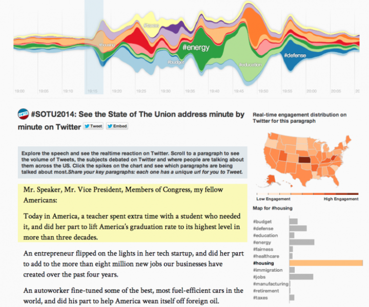
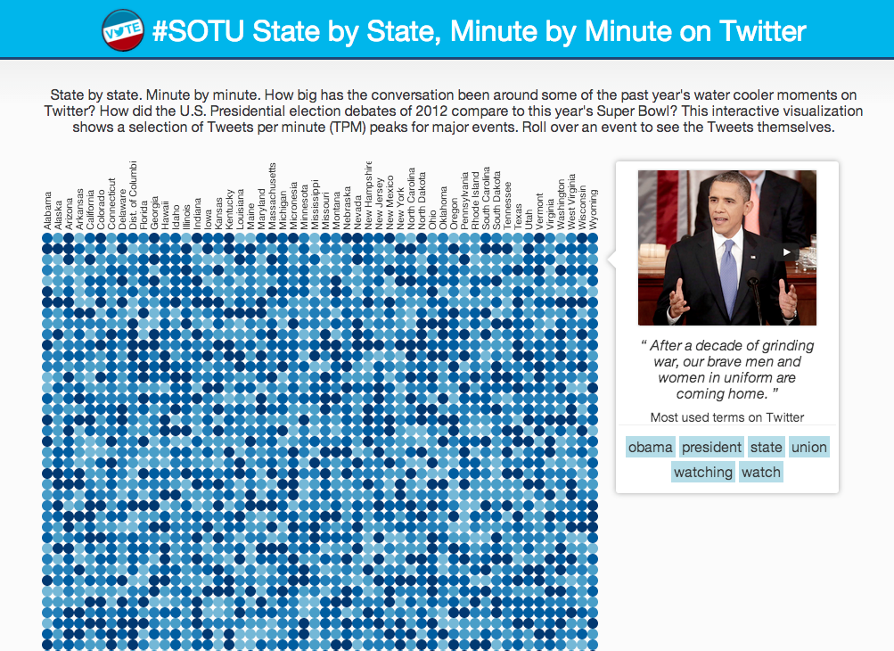
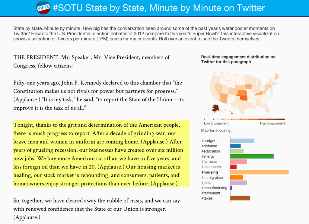
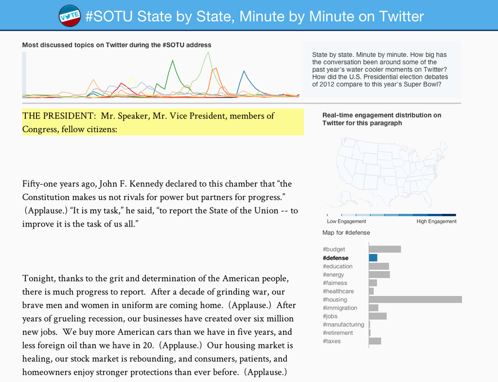
This project presents an interesting look into the play-by-play sentiments about Barack Obama’s 2014 State of the Union address. When hovering over a paragraph in the speech, the panels on the side and the top update to show relative frequency of tags, areas in the US with the highest engagement, and the flat uses of each corresponding hashtag. It was assembled by “the Twitter visual insights team,” led by data visualization scientists Nicolas Belmonte and Simon Rogers. (It is implied in their notes that the two of them might have been the whole team.) In the publication opennews.org, Belmonte and Rogers wrote an article themselves called “How We Made the SOTU Twitter Visualization.” They do not provide the dataset, but they do write in fairly technical detail how they went about developing the framework of the website, starting four weeks before the address. They knew they had to release the visualization around the time of the address, so they developed the website using a stand-in dataset of the tweets from 2013’s address. They started with the state frequency graph (top left), showing solely location-based engagement at minute-long intervals. From there, they began work on the front end and the bar graph of the most common hashtags in their dataset, arriving at the build in the top right. The finalized back-end build, shown at bottom left, also included a relative hashtag frequency graph that determined the paragraph breaks and timestamps used for the 2013 speech. Both during and after the 2014 SOTU address, Belmonte and Rogers swapped out the temporary dataset for the fresh timely tweets. After the visualizations reached their final forms, the data scientists “were up until 2:30am” adding timestamps to the paragraphs in the speech by hand, and the website was published.

If you have some background knowledge on JavaScript and data visualization, or if you want more technical details, their notes are a fun read.

For my fellow stats-minded people: I was wondering how they normalized the frequency data state to state, because if they had used a flat number of tweets per state the map would probably look more like a population density diagram. I also noticed that the states with smaller populations tended to swing much more violently, from not at all engaged to extremely engaged, while states like Texas and California never left the middle ranges of some engagement. The data scientists simply divided the number of tweets made by people in a state within a certain number of minutes by the number of total Twitter users in the state. So, a place with very few Twitter users, like North Dakota, doesn’t need as many tweets to make it look engaged. Additionally, they said they counted by tweet and not by user, so I would assume that if a user in West Virginia managed to post five times in two minutes, they would count that as five tweets in West Virginia instead of one engaged person in West Virginia. In my anecdotal experience, I have found that people tweeting about the SOTU address tend to tweet multiple times about different sections rather than just once, so I do wonder how different an identical frequency graph built on how many users tweeted per state within a certain amount of time would look. (If it looks the same, then we can assume each user is tweeting once, but if the colors on the map look lighter, then each user is probably engaging multiple times. If they look darker… we probably built the website wrong.)