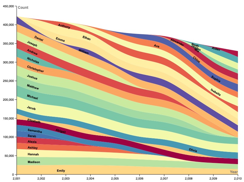
In my graph, I chose to focus on the relative total counts of baby names, rather than other factors such as rank and gender. I especially wanted to be able to look beyond the rank given to any particular name in order to see what that rank actually means. In this sense, I was aiming to showcase, rather than popularity, behavior of certain naming trends over time. I was curious to compare all the names side-by-side in order to see how this naming trends have ebbed and flowed over time, or perhaps have abruptly stopped or spontaneously began. Thus, I chose to showcase this using a streamgraph (area chart), as this was the only type of graph or chart that I found which could showcase so many different categories (names) of data in a way which ensured all of them were still individually discernible, but could also be easily compared side by side (as far as their counts go) over time. I am quite happy with this choice, as it is clear to see when each name grows or shrinks in popularity alongside all of the other names, and each name trend is obvious in the context of the entirety of its lifespan, which means that different behaviors during the lifespan of a single name can easily and intuitively be compared with each other and with those of other names.
To improve the clarity of my data visualization, I changed two things. Firstly, I changed the color gradient according to which different names were assigned different colors. Prior to doing this, over half of all of the names were assigned a similar (or even the same) shade of grey. I made sure to switch the color gradient to one that ensured each name not only had a different color that differentiated it from neighboring names, but that the data streams contrasted one another as much as possible to avoid confusion. Furthermore, I changed the position of the name labels from being “on point” (horizontal and oblique to the angle that the data streams flow) to “on path.” This ensured that the labels were as far from being stacked on top of one another as was possible, and more clearly aligned and correlated with each name stream, increasing the overall clarity of the graph.
My overall goal with this data visualization was, in consideration of Lin Winton’s lecture, to concisely present my data set. I figured that, since I was attempting to showcase so many data streams at once, I would need to make every other aspect of the graph as minimal as possible to properly communicating everything I was intending to, while still avoiding over-cluttering. As Lin illustrated during her presentation, this is easier said than done. However, I believe that, regardless of difficulty, while data visualization is often used misleadingly to support preeminent power structures, it can just as easily be used to peer behind their shrouds of surety. In the case of my graph, I aimed to do something similar with the baby name data, by illustrating not just a summary “ranking” of each name in every individual year, but a more accurate and continuous intuitive visual of how each name trend (the phenomenon itself) evolved over time. Ultimately, this function (seeing through the aspects of something which are commonly given in order to gain a deeper understanding of the fundamental phenomenon at play) is as applicable to obsolete baby names as it is to societal disharmony–and its dispelling.